Sustainability Assessment for Small Batch Manufacturing |
Analysis of textile manufacturing systems using material flow cost accounting (MFCA)
| Journal | Industry 4.0 Science |
| Issue | Volume 40, 2024, Edition 1, Pages 83-89 |
| Bibliography | Share | Cite | Download |
Abstract
Keywords
Article
In order to be able to operate sustainably and successfully despite relatively high costs for small manufacturing amounts, companies in the textile industry, and SMEs in particular, are faced with questions such as: How do I organize my manufacturing? What are the costs involved? How do I organize the processes? How does the manufacturing of small quantities affect the carbon footprint of my products? Numerous factors play a role here: minimum and maximum quantities per process step, waste and residues, plant size and configuration, energy type and costs, personnel costs and flexibility, and manufacturing planning and control, to name just a few.
Numerous specific studies have been carried out and models or procedures developed, not only for the textile industry [1]. However, there are no generic models that can be used across the sector (and beyond). It is precisely this gap that is closed with the methodology presented here and is already being used for the yarn and fabric manufacturing and textile finishing process stages.
Fabric manufacturing and weaving
For a better understanding, the methodology developed is illustrated below using the example of the textile process stage of fabric manufacturing on a dobby machine. In weaving, textile surfaces are produced using at least two thread systems (warp and weft). The weft threads are crossed at right angles with the warp threads. Dozens of weaving machines are usually used in weaving mills.
The fabric manufacturing process stage is divided into three sub-process stages: The warp manufacturing sub-process stage is divided into the creel assembly, warping, beaming and sizing processes as shown in Fig. 2. The resulting warp is drawn into the weaving harness in the pre-work sub-process stage. Each individual warp thread is first threaded through the eye in the corresponding heald shaft and then through the weaving reed. Then, in the weaving sub-process stage, the harness including the drawn-in warp is set up in the weaving machine by changing the harness. The actual weaving then takes place by inserting the weft yarns [2].
Material flow cost accounting – MFCA
The methodology presented here is based on material flow cost accounting (MFCA) in accordance with DIN EN ISO14051 [3, 4]. With MFCA, material and energy flows and their proportional costs, the personnel costs and the plant costs of the manufacturing systems as well as the greenhouse gas potential in companies can be holistically examined, balanced and evaluated [5]. Residues and waste as well as the set-up processes are taken into account in particular. For the examples described in this article, the Umberto LCA+ software tool from ifu Hamburg (now iPoint-systems GmbH, Reutlingen) was used for simulation.
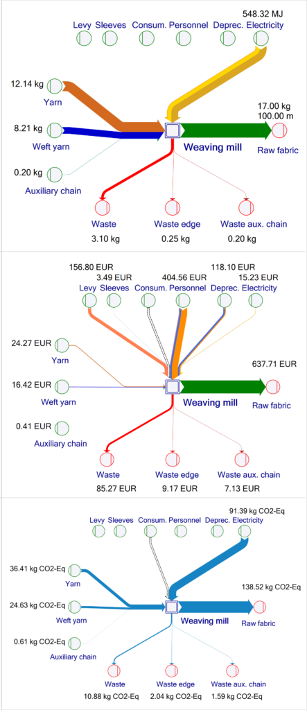
As shown in Figure 1, different views for material and energy flows (mass view, top), costs (cost view, middle) and carbon footprint (CO₂ view, bottom) can be generated on the basis of a common MFCA model. In addition to material, energy and personnel costs, the costs also include expenses for consumables (Consum.) and depreciation (Deprec.). These Sankey diagrams, in which the arrow thicknesses are proportional to the flows, make it possible to identify focal points and hotspots at a glance.
Simulation-based methodology suitable for SMEs
As described above, the methodology developed uses MFCA as a basis. The model parameters are recorded in an Excel form as a user interface, which is linked to the MFCA modelling and simulation tool via so-called LiveLinks. The five central aspects of the methodology (a to e) are described below.
(a) Hierarchical MFCA model structure per process stage
The process level models consist of a four-level hierarchical model structure. The lowest level models a generic process consisting of the set-up, manufacturing and cleaning sub-processes. Each of these sub-processes is modelled with different material, energy, equipment, personnel and auxiliary requirements. The two middle levels represent aggregations at plant level and workshop level. The respective textile process stage is located at the top level.
In concrete terms, using the example of the weaving process stage, this means that only the inputs of the material and energy flows are shown at the top level, with the products and waste flows as outputs, as shown in the mass view in Figure 1. The next level down, level 2, contains the sub-process stages of warp manufacturing, pre-work and weaving. At level 3, these are divided into processes. For warp manufacturing, for example, these are the processes for producing a warp, as shown in Fig. 2.
The lowest level in the model then forms a generic triple for each process, consisting of the set-up, manufacturing and cleaning sub-processes.
(b) Transformation of textile-specific product and process descriptions into the generic process model
The textile-specific product and process descriptions of the modelled process are recorded in the language of the SME experts in the Excel form and then transferred to the generic MFCA model parameters of the processes. For weaving, for example, the parameters for the description of a fabric, the yarn count and the warp and weft density, are provided by experts and then transformed into the generic material requirements for warp and weft yarn.
(c) Configurator for the basic design of alternative process routes
The desired process route is also described by the experts in the textile-specific process model and then transformed into the corresponding process route using the configuration in the Excel form. Figure 2 shows an example of this for the middle route with the warping/trees process sequence. Alternatively, manufacturing could be carried out directly from the creel (lower route in the figure) or with the process sequence warping/assembling (upper route). All possible routes are available in the model, but resources are only assigned to the active processes.

(d) Generic, preconfigured model components for each process
In addition, machine-specific setting parameters are used for each process in order to then transfer the productivity in generic form for the MFCA model. For example, the productivity of a weaving machine is described by experts in weft/min and must then be converted into the generic form kg/h.
In addition, the information on the yarn count is used, which is described in the textile-specific unit Tex (= gram/1000 m). The energy requirement in the model is also determined in kWh/kg from the electrical power of the machine and the productivity data described above. The relevant data on the fixed waste during set-up and cleaning as well as the variable waste portions during manufacturing are queried here and transformed into the generic form for the model. The same applies to the personnel expenses with the data fixed set-up and cleaning time and personnel costs/h as a basis. Similarly, the depreciation costs are transformed into the generic form €/kg using acquisition costs, depreciation period and shift calendar.
(e) Simulation of various scenarios
The data collection or user interface is implemented using a form in an Excel file. There is one line for each input parameter. The same applies to the transformed model parameters, which are transferred to the model by means of so-called LiveLinks. The values of the model parameters have already been calculated in Excel using the recorded input parameters, as described in Step b).
By separating the specific data for products and processes on the Excel data level and the MFCA model, different scenarios can now be calculated efficiently with one and the same model. For this purpose, all parameters of a described scenario are recorded in a column of the Excel file. By selecting the column of the desired scenario, the transformed process data is transferred to the predefined model parameters in the simulation tool. The model is then calculated using these parameters.
Validation was carried out by creating scenarios based on the company’s specific manufacturing orders and using the model to calculate the associated energy requirements and costs. The high level of agreement between the calculated and actual characteristic values in the company indicates a high quality of the model parameters.
Results of the simulation of various scenarios with different strategies
The results of the calculation can then be displayed in the three different views, as shown in Figure 1. The mass view shows the required resources as well as the associated manufacturing quantities and the waste proportions. The cost view shows the process costs of the resources used and allocates these to the end product and the waste proportions. This is a special feature of the MFCA method, as here the proportional process costs are explicitly allocated to the waste. The full cost view, which is not shown here, then allocates all shares of the waste streams to the end product, as these total costs are traditionally borne by the end product.
The same principle applies to the carbon footprint view, in which the associated CO₂ equivalents are shown. The Scope 3 emissions data [6, 7] of the materials and Scope 2 data of the electricity are used and calculated as a carbon footprint in accordance with DIN EN ISO 14040 [8] using the IPCC 2013 Life Cycle Impact Assessment method. Various manufacturing scenarios can thus be easily simulated and analyzed. This provides companies with decision-making support for the design and operation of manufacturing systems with regard to the resulting effects in terms of ecological and economic sustainability.
One of the exemplary questions examined was the effect of batch size on costs and the carbon footprint. Three different strategies were considered. In strategy 1, a scenario was defined and calculated for different batch sizes of the same article. The batch sizes varied from 10,000 running meters (= rm) down to the very small batch size of 100 rm. The results are shown in Figure 3.
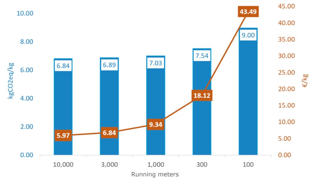
As the batch size decreases, the costs rise sharply and the carbon footprint per kg of fabric also increases. These increases are due to the fixed expenses in the set-up and cleaning sub-processes. These sub-processes still have to be carried out in all processes of each individual order. This involves the use of personnel and the generation of fixed quantities of material waste, as shown in Figure 2 for the warping and beaming processes.
A total of 2.5 kg of yarn is produced as waste. For large batch sizes, this proportion is low in relation to the total expenditure, but increases very sharply for small batch sizes. Personnel costs in particular have a much greater impact, as their fixed share is much more pronounced compared to the variable share during the manufacturing sub-process.
In these scenarios, the exact quantity of warp yarn required for the batch size was always produced. Strategy 1 can therefore already be considered critical from a batch size of 1,000 rm, as the specific costs already increase by more than 50% compared to 10,000 rm. Further scenarios were created and simulated in strategy 2. Here, a warp of 10,000 rm is produced, which is then set up in the weaving machine for each order. The warp remaining after the end of each order is stored in the harness until the next order.
This is only possible if the warp can be used for subsequent orders. In extreme cases, the harness is changed 100 times on the weaving machine with the warp retracted for small orders of 100 rm. This allows the costs and carbon footprint for warp manufacturing and drawing the warp threads into the harness to be kept to a minimum. The simulation of the scenarios that follow this strategy 2 shows the following result for the costs: For orders with a batch size of 100 rm (1,000 rm), approx. 64% (27%) of the costs and 18% (2%) of the carbon footprint are saved compared to strategy 1.
As strategy 3, the elimination of permanent set-up processes on the weaving machine was also examined. The large 10,000-rm warp always remains in the weaving machine until it is completely used up. This means that the weaving machine is blocked for processing other orders. Nevertheless, the costs for depreciation and air conditioning are incurred during downtime. However, there are no set-up costs as the warp remains in the machine. This strategy is economical for batch sizes of 1,000 rm up to a downtime of approx. 40 % in relation to the productive time of the weaving machine. With the very small batch size of 100 rm, the downtime can even be up to 83%.
Conclusion from the comparison of different strategies
The comparison of the scenarios with different strategies is an example of how economically and ecologically sustainable textile manufacturing is possible even with small batch sizes. The prerequisite for this is to develop the different fabrics in such a way that they can be produced with the same warp. Different designs can be implemented by using different weft yarns and fabric weaves.
The quantitative data and results in these examples should not be regarded as absolute and typical characteristic values. The sensitivity of these parameters is strongly influenced by the yarns used, the fabric construction, the machine technology used across the entire process chain and the labor cost rates. As the weaving process is an energy-intensive process, the carbon footprint of the product reacts extremely sensitively to the specific carbon footprint of the electricity used.
The characteristic values for the carbon footprint are extremely different for green electricity with a high proportion of renewable energy on the one hand and electricity from brown coal on the other. The yarn count also influences the manufacturing time and therefore has a significant impact on energy requirements and personnel costs.
The results presented here clearly show the added value of a hierarchical and generic model and the ability to create scenarios. These make it possible to quickly and effectively determine parameters for specific framework conditions and issues. For example, the methodology was used as part of a concept for communicating sustainability information [9]. It was also used to investigate sustainability data in a decision support system [10]. Current research topics include determining the carbon footprint of materials used, especially when taking Scope 3 into account [6], and modelling complex supply chains.
This article was written as part of the project “Profitable small-scale textile manufacturing – ReKleT” (IGF project 20660 N) [11], which was funded by the Federal Ministry of Economics and Climate Protection as part of the program for the promotion of joint industrial research (IGF) on the basis of a decision by the German Parliament.
Bibliography
[1] Seibold, J.; Weiß, M.; Mirosnicenko, A.; Stipic, N.; Schneider, R.; Brenner, S.: Nachhaltigkeitspotenziale von Microfactories für textile Produktionsnetzwerke erschließen, Schlussbericht Vorhaben-Nr. IGF 20534 N, DITF Denkendorf (2022).[2] Bauder, H. J.; Stellmach, D.; Wolfrum, J.: Technologische und organisatorische Optimierung von Kett- und Artikelwechselvorgängen in der Schaftweberei bei Einsatz moderner Handhabungsgeräte, Schlussbericht AiF 12858, DITF-Denkendorf (2003).
[3] DIN EN ISO 14052:2018 Umweltmanagement – Materialflusskostenrechnung – Leitfaden zur praktischen Anwendung innerhalb der Lieferkette (2018).
[4] ISO 14053:2021 Umweltmanagement – Materialflusskostenrechnung – Anleitung zur praktischen Umsetzung in KMUs (2021).
[5] RKW Rationalisierungs- und Innovationszentrum der Deutschen Wirtschaft e. V., Materialflusskostenrechnung – Effizient mit Ressourcen umgehen. Faktenblatt 2/2011, URL: www.rkw-kompetenzzentrum.de/innovation/faktenblatt/effizient-mit-ressourcen-umgehen-materialflusskostenrechnung, Abrufdatum 14.11.2023.
[6] Corporate Value Chain (Scope 3) Accounting and Reporting Standard, World Resources Institute and World Business Council for Sustainable Development (2011). URL: ghgprotocol.org/sites/default/files/standards/Corporate-Value-Chain-Accounting-Reporing-Standard_041613_2.pdf, Abrufdatum 14.11.2023.
[7] Technical Guidance for Calculating Scope 3 Emissions., World Resources Institute & World Business Council for Sustainable Development (2013). URL: ghgprotocol.org/scope-3-technical-calculation-guidance#supporting-documents, Abrufdatum 22.03.2023.
[8] DIN EN ISO 14040:2021 Umweltmanagement – Ökobilanz – Grundsätze und Rahmenbedingungen (2021).
[9] Stellmach, D.; Weiß, M.; Seibold, J.; Tilebein, M.: Towards a Digital Workflow Solution for Cradle-to-Gate Sustainability Information in Textile Value Chains. In: Proceedings 3rd Conference on Production Systems and Logistics, Vancouver 2022. DOI: doi.org/10.15488/12155.
[10] Weiß, M.; Winkler, M.; Seibold, J.; Grau, G.: Welchen Beitrag zur Nachhaltigkeit kann die Digitalisierung liefern? Ein Ansatz zur Bewertung der Digitalisierung in der Textilproduktion hinsichtlich ökologischer und ökonomischer Nachhaltigkeit. In: Industrie 4.0 Management (2023) 2, S. 25-28.
[11] Stellmach, D.; Seibold, J.; Stipić, N.: Entwicklung einer simulationsbasierten Methode zur Unterstützung bei Gestaltung und Organisation von Produktionssystemen zur rentablen Kleinmengenherstellung von Textilien, Schlussbericht Vorhaben-Nr. IGF 20660 N, DITF Denkendorf (2022).
Your downloads
You might also be interested in