Production Control in Space |
An AI-supported approach for industry in orbit
| Journal | Industry 4.0 Science |
| Issue | Volume 41, 2025, Edition 6, Pages 22-29 |
| Bibliography | Share | Cite | Download |
Abstract
Keywords
Article
In an increasingly competitive environment, companies must explore new production methods. The main driver here is cost, which is fueling the current digital transformation but also leading companies to relocate their production to more economically favorable areas. In the near future, some experts foresee the first production facilities in space, or more precisely, in orbit. In just a few years, goods such as medicines, semiconductor crystals, and organoids (organ-like pieces of tissue) could be manufactured in this way [1].
The first in-orbit production is likely to take place in three to five years, as research into the required space capsules advances swiftly and innovators such as Elon Musk and Jeff Bezos manufacture powerful rockets [2]. The company Starship, for example, aims to manufacture completely reusable rockets with a capacity of several hundred tons, which will significantly reduce the cost of space travel. By way of comparison, sending one kilogram into orbit costs around $2,700 with the current Space X Falcon 9. Starship aims to bring this down to less than $500. Flying to the ISS or the moon costs $20,000-40,000 and $1 million per kilogram, respectively [3].
Every gram of weight sent into space must be carefully considered, for obvious economic (and ecological) reasons. This presents a dilemma: you want to establish production in space that meets standards on Earth. However, the costs of transporting the necessary systems, robots, peripherals, etc. will remain very high in the coming years, which could mitigate any advantages.
One potential cost lever is to forego local, intelligent edge systems such as IoT edge devices or NVIDIA Jetson platforms and instead turn to centralized production control from Earth. At the very latest when using artificial intelligence (AI), the systems will have to be controlled from Earth, as high costs would otherwise be incurred for the provision of the necessary computing power in space.
Production control from Earth will thus be virtually unavoidable in coming years. However, this has the disadvantage that latency hinders the real-time capability of robots and systems. If production is not located in orbit but on the Moon (or Mars), for example, this latency is significantly higher. This means, for example, that transport systems or robots controlled from Earth can only react to their environment with a delay. The news of an obstacle ahead and the subsequent reaction take several seconds, which may be too late in some circumstances. In such cases, one can no longer speak of real-time capability.
Mathematical estimation methods, such as those used in radar technology to determine an aircraft’s exact position and flight path, can help [4]. These methods can also be used to control a device in space in near real time and with greater accuracy, depending on the degrees of freedom that a system has (e.g., if it moves freely or along a predetermined route).
A model for (real-time) production control of systems in space
To understand how mathematical functions help enable real-time production control, let’s use a simple example: You are driving your car into a tunnel and the GPS signal is lost. You want to take the next exit in the tunnel. How does the navigation device know where you are? It uses data from the vehicle sensors and the last known position to determine (approximately) where you are.
In principle, it could calculate your location at any time based on your speed and last position. But this only works in a perfect world, because sensors are subject to measurement inaccuracies, interference occurs during data transmission to the microcontroller, or deviations occur in other places. This leads to inaccuracy in what is actually a simple piece of information: “speed”.
In this simple model, one could now use so-called estimated values to eliminate disturbances and associated “distortions”. This works quite well in this one-dimensional case [5][6], but a driverless transport system moving freely in space, for example, is already a multidimensional case not accurately captured with simple estimated values.
The same applies to our latency time. Although factors such as distance and weather conditions make it fairly constant, it is subject to a certain degree of inaccuracy. The following histogram illustrates this with an example: Although the maximum expected latency time is around three seconds, deviations in the millisecond range do occur. These deviations are called variance or “noise”. It is striking that the deviations are approximately normally distributed. This allows specific mathematical methods to analyze and correct the measured values.
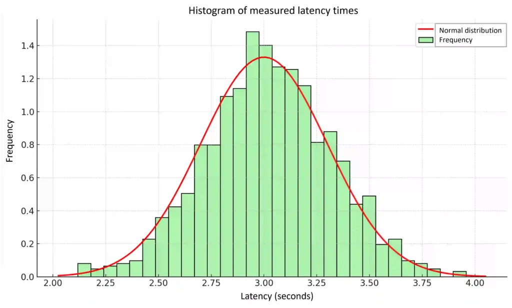
In order to perform reliable calculations despite variance or noise, the “strength” of the noise must first be determined. This is determined individually for each sensor and taken into account in the calculations accordingly. The mean value is used—the expected value, e.g., the speed—as well as the variance of the normal distribution, which indicates how certain or uncertain the estimate is. As a general rule, the smaller the variance, the greater the confidence in the measured value. A sensor with absolute precision would theoretically have a variance of 0—a state that never occurs in reality [7].
In our navigation device example, we assume that the GPS signal has been lost and that the navigation device is unsure of its current location. Accordingly, the variance or uncertainty about the exact position is very high. In order to estimate a position nonetheless, other available data would be used, e.g., the measured speed. However, the speed sensor also has a certain variance and is therefore also subject to uncertainty.
Combining the uncertainties of the navigation device and the speed sensor yields a better result, allowing the navigation device to determine a more accurate current position. The navigation device knows “approximately” where you are and the sensor knows “approximately” how fast you are traveling, which allows for a relatively accurate statement in combination (this can be observed in everyday life: position determination in a tunnel is usually still very precise).
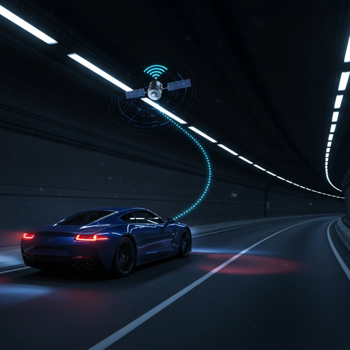
This approach was described by R. Kalman as early as 1960 and helped with the first moon landing [8]. Using the so-called Kalman filter, all you do is calculate a future position from the current position and check it (e.g., by taking measurements). These calculations and checks allow us to find the appropriate parameters to compensate for the “noise”, i.e., the variance. If the predicted values are close to the values measured afterwards, then the Kalman parameters are very accurate. In our example: If the car exits the tunnel at exactly the right moment (and has a GPS signal again, which enables location determination), then the estimation parameters are very well chosen. Otherwise, the parameters would be adjusted.
In our example, we are moving in a one-dimensional (maximum two-dimensional) direction; the example has a low level of complexity. However, this forms the basis for the real-time control of significantly more complex production facilities in space. The position determination of a transport system on a planet depends not only on the respective distance, but also on the respective rotation, which is also subject to fluctuation. This gives us a complex system with several uncertainties, but we can easily reduce or even completely eliminate these by applying the mathematical model.
Development environments such as MATLAB include these Kalman functions, which makes creating and implementing such a mathematical model very easy [9]. Systems for controlling these devices in space could therefore be expanded by mathematical functions at low cost and with little effort.
That said, such systems are becoming increasingly complex and navigation and control are expected to become more autonomous with time. AI approaches can help: machine learning can assist in determining parameter values, for example, or a digital twin of production in space can be created.
AI can also be helpful in the case of fault-prone signal processing [10] or in dealing with parameters for target positions within an image plane in order to predict them. In the latter case, the position of the target is recorded in each iteration to predict the positions one step ahead [11]. This can also improve the position determination of driverless transport systems (in space). In principle, Kalman filters and their use in space production can themselves also be improved by AI.
Machine learning to improve Kalman filters in complex systems
As already described, the increasing trend toward machine learning algorithms not only creates new possibilities for AI-supported position determination but also makes Kalman filters and associated parameters more accurately predictable. The comparison of “estimated” and “measured” data in the application of Kalman filters represents a (historical) database, which can be used to train corresponding AI algorithms. These can then reveal hidden patterns in the relationship between the estimated and measured data.
This does not work as accurately during dynamic scenarios brought about by system control or the routing of transport systems by AI. The parameters of the Kalman filters estimated by AI algorithms can quickly become outdated, as they are based on “past” data. However, an additional learning model can overcome this challenge by modifying the parameters according to the new conditions, even if these are caused by AI and are therefore sometimes difficult to predict [12].
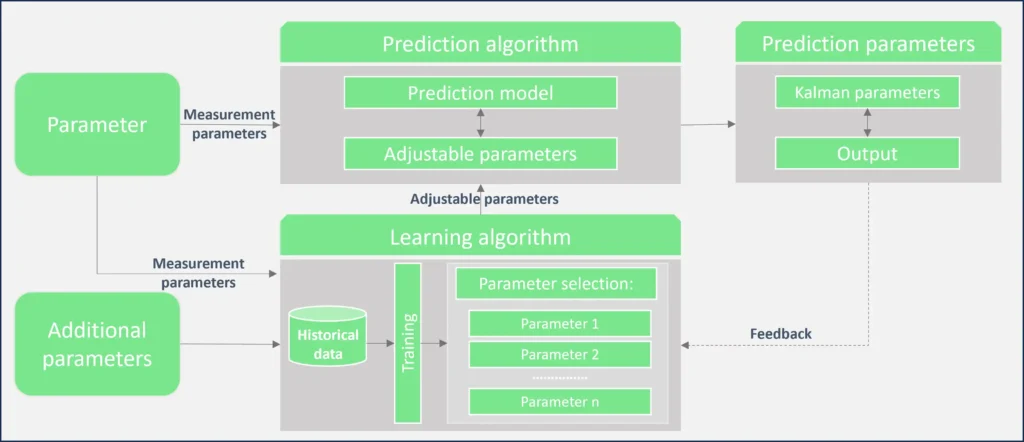
This more advanced model consists of a prediction module and a learning module. The prediction module receives the measured and estimated values, such as the location and speed of a transport system in space. The module then determines the parameters of the Kalman filter and the exact location [13]. The learning module uses the same parameters as the prediction module, supplemented by additional influencing factors. Based on historical data and the associated parameters, the learning module calculates so-called “tuning” parameters that help the prediction module determine the optimal Kalman parameters. The combination of both modules enables precise determination of the status data and real-time production control even given longer latency times.
The rapid progress in the field of deep learning algorithms and related technologies also has a positive effect on our approach. The targeted use of modern methods such as deep belief networks (DBNs), a hierarchically structured form of neural networks that recognize complex patterns in data [14], or deep extreme learning machines (ELMs), which enable particularly fast learning processes through randomly initialized hidden layers, can significantly improve prediction accuracy [15].
Classic machine learning methods such as classification and regression trees (CARTs) can also be used [16]. These structured decision-making processes are represented in the form of tree diagrams, making them suitable for both classification and regression tasks. Support vector machines (SVMs), which are designed to find optimal separation lines (or hyperplanes) between different data classes, also make an important contribution to precise modeling [17].
All these methods are integrated into the learning module and trained using historical data. The aim is to derive so-called tuning parameters, which in turn increase the accuracy of the Kalman parameters used in the prediction module. In this way, the overall system can respond more robustly and reliably to dynamic changes in the input data.
In summary, the presented system architecture, consisting of a learning and a prediction module, represents a more precise approach for estimating variables using Kalman filters. By integrating modern machine learning methods into the learning module, adaptive tuning parameters can be generated based on historical data, enabling continuous optimization, even when using AI, e.g., for system control. This allows for increased accuracy, even in highly dynamic application scenarios such as those that can arise from the aforementioned AI-based control or system routing.
The promise of production in space
Production in space already appears very promising in near-Earth spheres. At the same time, the transport of the necessary production equipment still involves enormous costs. These can be reduced by controlling production from Earth, but latency and other uncertainties hinder real-time control at such great distances, which can lead to accidents.
In very simple cases, there are mathematical models that can provide accurate predictions. However, since production in space is complex, with many disturbances and uncertainties, and since the use of AI will make these models even more complicated in the future, the use of statistical methods such as the Kalman filter is essential. In these complex situations, machine learning algorithms can help to accurately determine the necessary parameters. Using a learning prediction model, these can be determined very accurately and even optimized during the learning process.
Although machine learning and necessary peripherals do incur additional costs, these are falling steadily and more and more training data sets are becoming available, so that this approach will also prevail in terms of cost in the long term. Compared to (falling) transport costs, they represent the significantly more cost-efficient solution in the coming years and are a central component of production in space.
Bibliography
[1] Weinzierl, M.; Rosseau, B.: Space to Grow: Unlocking the Final Economic Frontier. USA: Harvard Business Review Press, 2025. ISBN 978-1647827175.[2] Roettgen, R.: To Infinity: The New Space Economy, independently published, 2024. ISBN 979-8864261378.
[3] SpaceX: Capabilities and Services Falcon 9. URL: https://www.spacex.com/vehicles/falcon-9/, accessed 15.04.2025.
[4] Hall, D. L.; McMullen, S.: Mathematical Techniques in Multisensor Data Fusion. Artech House, 2004. ISBN 978-1580533355.
[5] Asquith, C. F.: Weight selection in first-order linear filters. Technical report. Army Inertial Guidance and Control Laboratory Center, Redstone Arsenal, Alabama, 1969. DOI: 10.21236/ad0859332.
[6] Tenne, D.; Singh, T.: Optimal Design of α-β-(γ) Filters. In: Proceedings of the American Control Conference, 2000. DOI: 10.1109/ACC.2000.877043.
[7] Welch, G.; Bishop, G.: An Introduction to the Kalman Filter, University of North Carolina at Chapel Hill, 2006.
[8] Kalman, R. E.: A New Approach to Linear Filtering and Prediction Problems, Transaction of the ASME. In: Journal of Basic Engineering (1960), pp. 35-45.
[9] MATrix LABoratory: Kalman Filter. URL: https://www.mathworks.com/discovery/kalman-filter.html, accessed 15.04.2025.
[10] Zhang, H. et al.: An updated method for digital twin multi-dimension models. In: Robotics and Computer-Integrated Manufacturing 80 (2023).
[11] Stanciu, R.; Oh, P. Y.: Human-in-the-loop camera control for a mechatronic broadcast boom. In: IEEE/ASME Trans. Mechatron (2007) 12, pp. 41-52.
[12] Khan, J.; Kim, K. A.: Performance Evaluation of the Alpha-Beta (α-β) Filter Algorithm with Different Learning Models: DBN, DELM, and SVM. In: Appl. Sci. (2022) 12, p. 9429.
[13] Khan, J. et. al.: An Improved Alpha Beta Filter Using a Deep Extreme Learning Machine. In: IEEE Access 9 (2021), pp. 61548-61564. DOI: 10.1109/ACCESS.2021.3073876.
[14] Phyo, P. P.; Jeenanunta, C.: Daily Load Forecasting Based on a Combination of Classification and Regression Tree and Deep Belief Network. In: IEEE Access (2021) 9, pp. 152226-152242.
[15] Fayaz, M.; Kim, D.: A prediction methodology of energy consumption based on deep extreme learning machine and comparative analysis in residential buildings. In: Electronics (2018) 7, p. 222.
[16] Lewis, R. J.: An introduction to classification and regression tree (CART) analysis. In: Proceedings of the Annual Meeting of the Society for Academic Emergency Medicine, San Francisco, CA, USA, May 22–25, 2000; Volume 14.
[17] Osuna, E.; Freund, R.; Girosi, F.: An improved training algorithm for support vector machines. In: Neural Networks for Signal Processing VII, Proceedings of the 1997 IEEE Signal Processing Society Workshop, Amelia Island, FL, USA, September 24–26, 1997; IEEE: Piscataway, NJ, USA, 1997; pp. 276–285.
Potentials: Innovation Profitability
Solutions: Production Control Risk Management
You might also be interested in