Predictive Manufacturing |
An intelligent monitoring system to detect anomalies in 3D printing
| Journal | Industrie 4.0 Management |
| Issue | Volume 39, 2023, Edition 1, Pages 27-31 |
| Open Access | https://doi.org/10.30844/I4SE.23.1.88 |
| Bibliography | Share | Cite | Download |
Abstract
Article
Selective laser melting
Selective Laser Melting is used in industry to produce metal components and is becoming increasingly important in the manufacturing industry. It is an additive manufacturing process in which a bed of metal powder is applied in even layers to a component platform and melted using a laser. This makes it possible to produce components with comparatively high individual geometric requirements. The process involves repeated heating and cooling cycles, during which the components are subjected to constant high stresses.
To ensure a high quality standard, defective printed layers should be avoided. Defective layers have issues such as pores, cracks or unevenness, which lead to quality-reducing properties. The components or test components are tested for tensile or compressive strength only after printing to ensure the quality of the components. If the test results are negative, the component is analyzed and printed again with optimized process parameters, making the process very costly and time-consuming [1].
Methodology
To enable detection during the printing process itself, two methods are used: an autoencoder and principal component analysis. Both methods obtain greyscale images generated by Siemens, which show the printed layers of the component from a bird’s eye view.
Pre-processing of the greyscale images
In the field of machine learning, data pre-processing is an essential step. Neural networks are only as good as the quality of the data they predict. The Siemens example dataset contains an image of the entire component platform per layer. In this particular print job, nine components with different geometric dimensions are created at the same time, so they have to be separated in the greyscale image. It is necessary to improve the visibility, contrast and brightness of the clipped images.
The colors of the images are converted to the so-called LAB color model, while Contrast Limited Adaptive Histogram Equalization (CLAHE) improves the brightness channel. All three channels are then combined [2].
Artificial neural networks model the functioning of the human brain and simulate learning using neurons. They are used, for example, in image recognition, where they have achieved groundbreaking milestones. A summarizing overview of how artificial neural networks work and successful applications, especially but not exclusively in imaging, is given by Z. Li et al. [3].
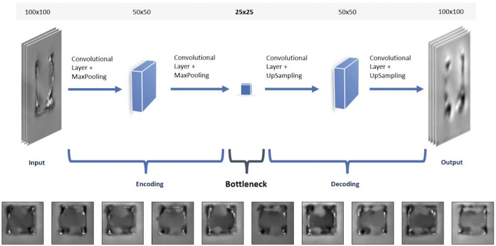
Figure 1: Autoencoder that receives the separated components as input, transforms them to a low-dimensional vector space in the encoding step and back-transforms them in the decoding step, thus reconstructing the input. Below are examples of greyscale images of the individual layers.
Autoencoder
Autoencoders are neural networks that consist of two phases:
An autoencoder reduces the dimension of an input in the so-called encoding step and reconstructs the original input in the so-called decoding step, as shown in Figure 1.
After the encoding step, a compressed representation of the input is available that contains all the information to reconstruct the input. The autoencoder learns transformation functions in differently dimensioned vector spaces.
This is done by training an autoencoder on a set of images. The trained autoencoder can reconstruct similar images without having seen them before. Early stopping is used to determine the number of epochs for training. This automatically stops the training of the autoencoder when the loss of test data between epochs ceases to vary significantly. The loss serves as a quality criterion of a model and is calculated from a corresponding loss function.
Model error is then calculated from mean square error. Using early stopping also prevents overfitting of the model to the training data [4]. The number of epochs depends on the design and training of the autoencoder.
The idea is to use images to train the autoencoder on a non-defective print. In particular, other images that also come from a non-defective print should be able to be reconstructed well, while images from faulty print layers are less well reconstructed. These deviations in the images are measurable and visualized in the demonstrator, as shown in Figure 2. During printing, the deviation is visible for each layer. If there are a certain number of layers with high deviations, printing can be stopped because quality degradation can be expected.
After data pre-processing and autoencoder training, intelligent monitoring of the print job is possible. Irregularities that indicate defective layers are called anomalies. Faulty layers indicate a reduction in component quality and are avoidable. Using the autoencoder and the reconstructed images, anomalies can be detected in the printing process. By training on high quality printed layers, the autoencoder cannot reconstruct defective layers well, increasing the reconstruction error and making anomalies visible.
Mean square error (MQA) is proposed to calculate the reconstruction error:
Reconstructionerror=(originalimage-reconstructedimage)2 (1)
MQA is a standard metric in many machine learning applications. In the best case, the reconstruction error converges to 0, which indicates high-quality printed layers [5, 6].
Principal component analysis
Principal component analysis is a well-known method of linear dimension reduction [7]. Calculations are used to determine the so-called principal components of the data. These are exactly the characteristics of the data that mainly define it. Correlations between variables are used to reduce the data set to less uncorrelated principal components [8]. In this case, the 3D printed images are to be reduced to two dimensions (an image has 100 x 100 pixels or dimensions in the input).
The goal is a 2-dimensional representation of the images as points of a cluster in the diagram. Defective layers are identified by the scattering of these points in the diagram. The distance between the scattered points is determined by calculating a cluster center. Neighboring layers should be very similar, so ideally the image of a layer will always be close to the cluster centre.
Decision support application
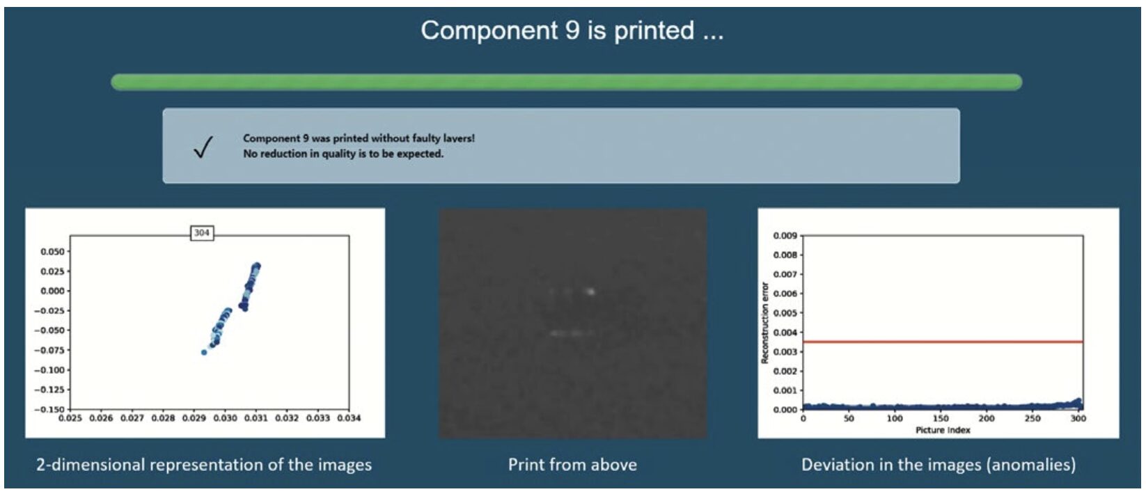
Both methods are visualised in the demonstrator as shown in Figure 2.
The left-hand side of Figure 2 shows the image features. These features are projected onto a 2-dimensional vector space using the coupling of the autoencoder and principal component analysis. The encoding step in the autoencoder transforms the images into a 25 x 25 vector space. Principal component analysis then reduces this vector space to a 2D vector space to map the existing image features onto the points. Ideally, this will produce two clusters, thus indicating a good print. The origin of the two different clusters can be traced back to the different exposure requirements due to the position of the coater in the press. The printed layers are alternately exposed brighter and slightly darker. Two clusters are visible, with the points of one cluster moving downward due to the pyramidal geometry.
The topology of the points within the cluster can be traced back to the pyramidal geometry. On the right hand-side of Figure 2, the reconstruction error of the autoencoder is calculated. This allows the progress of the printing process to be assessed against a threshold. Both monitoring parameters can independently detect irregularities that indicate errors in the printing process and require manual intervention.
Analysis of the components and results
An empirical threshold can be defined that separates the printed layer into defective or non-defective, and decisions can be made about how to proceed. Anomalies are detected as soon as the reconstruction error exceeds the threshold, otherwise it is safe to continue printing.
The user is free to adjust this threshold upwards or downwards, for example to update component quality standards. The number of outliers gives an indication of the component quality. For demonstration purposes, the following rules, which result from professional evaluation of components and image sequences, can be defined:
- The component is considered to be error free if no reconstruction error is above the threshold.
- The component is considered minimally defective if one or two reconstruction errors are above the threshold.
- The component is considered potentially faulty (and should be checked manually) if three or four reconstruction faults are above the threshold.
- The component is considered to be severely defective if there are at least five reconstruction errors above the threshold.
If the available components are analyzed using this set of rules, the following evaluation results:
- Component 1: severely defective (13 defective layers)
- Component 2: slightly defective (2 defective layers)
- Component 3: slightly defective (1 defective layer)
- Component 4: severely defective (50 defective layers)
- Component 5: slightly defective (1 defective layer)
- Component 6: slightly defective (1 defective layer)
- Component 7: potentially defective (4 defective layers)
- Component 8: faultless (0 defective layers)
- Component 9: faultless (0 defective layers)
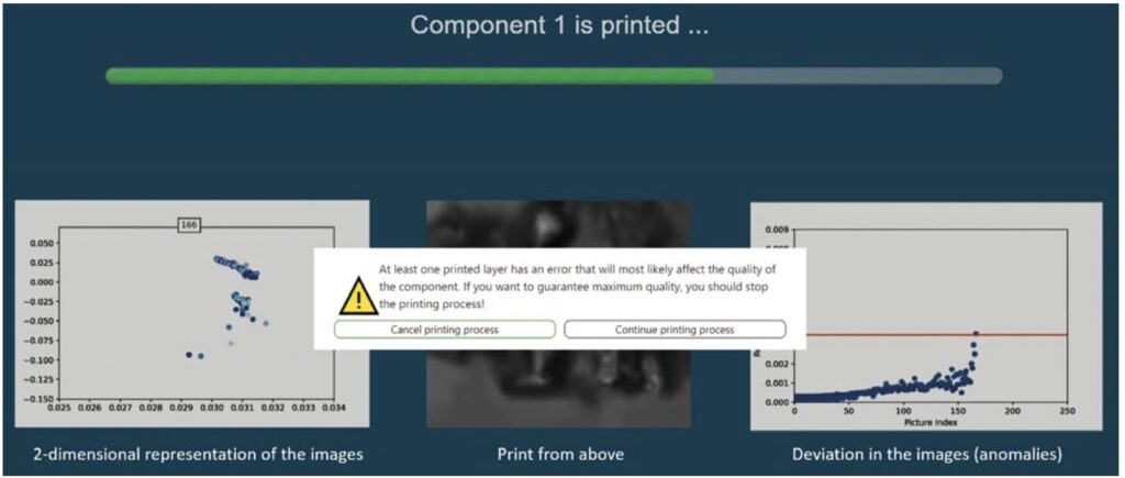
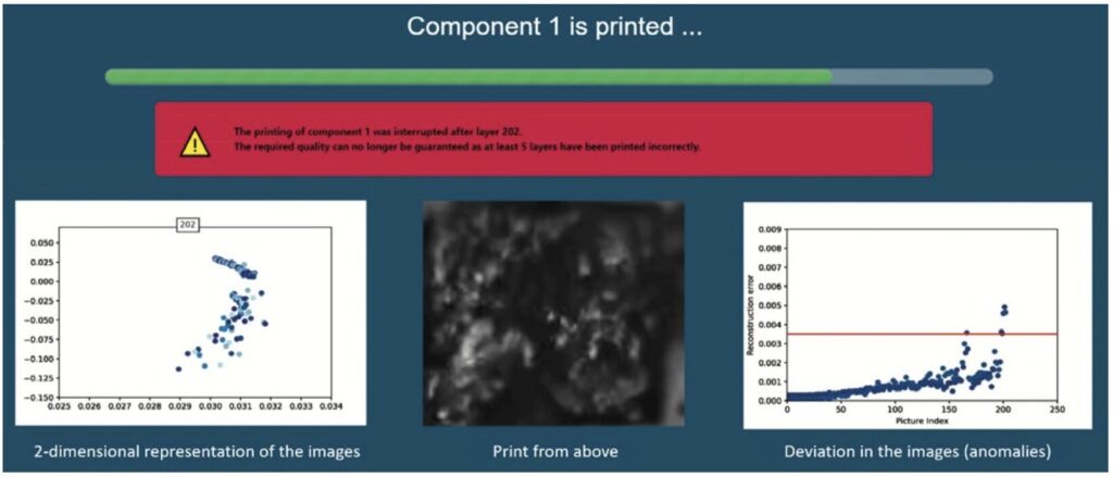
In addition, the authors propose to have the monitoring system give a warning for each defective printed layer, with the option to stop or continue the printing process. Furthermore after five consecutive defective layers, the print job stops automatically. Both cases are shown in Figure 3 and Figure 4, respectively. For component 1 the process is stopped after 745 layers and for component 4 after 684 printed layers.
Summary and outlook
Automatic detection of faulty layers during the printing process using an intelligent monitoring system saves time and resources. To achieve this goal, greyscale images were generated and pre-processed. The training of an autoencoder is based on two high quality components. The difference between the original image and the reconstructed image is used to identify anomalies. If one component has too many outliers, the printing process can be stopped early to save material. In addition, the image features of each layer can be reduced to two dimensions. This allows these features to be visualized in the greyscale image, providing a graphical representation of the printing process. This can be used to identify characteristics and similarities between printing processes.
For future work, it would be interesting to evaluate the approach with other components. Other component geometries could also be analyzed. For this, it is necessary to train the autoencoder with components of varying geometric compositions. To apply this approach in practice, it is possible to read and process the greyscale images of each layer in real time. The speed of printing and the performance of the application are important here and have not yet been considered in the current work. It would also be conceivable to train an artificial neural network to classify defective or non-defective layers.In addition, other classification algorithms such as random forest or a support vector machine could be used.
Due to high resource consumption and post-print quality control (printing a part can take anywhere from several hours to several days), the standard process is comparatively inefficient. Automated early detection of defective layers will make 3D printing more profitable and sustainable.
3D printing with integrated quality control requires minimal manual intervention. Using the methods presented, it will be possible in the future to intelligently monitor complex industrial systems such as 3D printing. Production processes can be continuously optimized and the need for human supervision of individual machines will be eliminated.
Intelligent analysis and visualization can be extended to heterogeneous sensor data streams from production processes. This will make it possible to detect faults in different production parameters and processes. To this end, the development of hybrid models for the thermal simulation of melting processes during 3D printing is being researched at Leipzig University and by Scads.AI [9]. In particular, mapping of physical relationships such as ordinary or partial differential equations are coupled with classical machine learning methods to generate data-driven, interpretable predictive models. This results in novel intelligent systems [10] [11].
This article was written as part of the project “TWIN-Transformation of complex product development processes into knowledge-based services for generative manufacturing”, which is funded by the German Federal Ministry of Education and Research under the reference number 02K18D050 ff.
Bibliography
[1] Bremen, S.; Meiner, W.; Diatlov, A.: Selective Laser Melting- A manufacturing technology for the future? In: Laser Technik Journal, (2012), pp. 33-38.[2] Chang, Y.; Jung, C.; Ke, P.; Song, H.; Hwang, J.: Automatic contrast-limited adaptive histogram equalization with dual gamma correction. IEEE Access (2018), 6: pp.11782-11792.
[3] Li, Z.; Liu, F.; Yang, W.; Peng, S.; Zhou, J.: A Survey of Convolutional Neural Networks: Analysis, Applications and Prospects, IEEE Transactions on Neural Networks and Learning Systems (2021), Volume 33: pp. 6999 -7019.
[4] Yao, Y.; Rosasco, L.; Caponnetto, A.: On Early Stopping in Gradient Descent Learning, Constructive Approximation, (2007): pp. 289-315.
[5] Zimmerer, D.; Kohl, S.; Petersen, J; Meier-Hein, F.; Isensee, K.: Context encoding variational autoencoder for unsupervised anomaly detection. CoRR (2018): pp. 1-13.
[6] An, J.; Cho, S.; Variational autoencoder based anomaly detection using reconstruction probability. Special Lecture on IE (2015), pp. 1-18.
[7] Wang, Y.; Yao, H.; Zhao, S.: Auto-encoder based dimensionality reduction. Neurocomputing (2016), pp. 232-242.
[8] Dette, H.; Härdle, W.; Principal component analysis, Multivariate Analysemethoden von Andreas Handl, Springer Verlag (2010), pp. 126-147.
[9] Uhrich, Benjamin; Schäfer, Martin; Theile, Oliver; Rahm, Erhard (2023): Using Physics-Informed Machine Learning to Optimize 3D Printing Processes. In: Joel Oliveira Correia Vasco, Henrique de Amorim Almeida, Anabela Gonçalves Rodrigues Marto, Carlos Alexandre Bento Capela, Flávio Gabriel Da Silva Craveiro, Helena Maria Da Coelho Rocha Terreiro Galha Bárt et al. (Eds.): Progress in Digital and Physical Manufacturing. Cham: Springer International Publishing (Springer Tracts in Additive Manufacturing), pp. 206-221.
[10] Bauer, M; Uhrich, B; Schäfer, M.; Theile, O.; Augenstein, C; Rahm, E.: Multi-Modal Artificial Intelligence in Additive Manufacturing: Combining Thermal and Camera Images for 3D-Print Quality Monitoring. In: Proceedings of the 25th International Conference on Enterprise Information Systems – SCITEPRESS – Science and Technology Publications; 2023. pp. 539-546.
[11] Uhrich, Benjamin; Hlubek, Nikolai; Häntschel, Tim; Rahm, Erhard (2023): Using differential equation inspired machine learning for valve faults prediction. In: 2023 IEEE 21st International Conference on Industrial Informatics (INDIN). 2023 IEEE 21st International Conference on Industrial Informatics (INDIN). Lemgo, Germany, 18.07.2023 – 20.07.2023: IEEE, pp. 1-8.
Your downloads
You might also be interested in