Parameter Optimization for a Brine Injector

Cooked ham production process 

According to the guidelines for meat and meat products, the term ham, also in word combinations, is only used for products of at least superior quality. Only untrimmed meat cuts such as topside, silverside, thick flank and/or haunch are used in the production of ham [1].

To produce cooked ham, the aforementioned meat cuts are processed during wet curing using the muscle injection method. In this process, brine is injected into the muscle meat under pressure, using injectors. This ensures that the brine diffuses evenly. Curing has different effects on the food. It inhibits microbiological spoilage and has a coloring and aroma-building effect on the product. This is followed by the mechanical process of “tumbling”, which loosens the tissue.

This releases muscle protein so that the slices of cooked ham can later be held together. The pieces of meat are then placed in molds or stuffed into casings, cooked at temperature and, finally, subjected to a cooling process in order to achieve microbiological safety. Depending on the end product, the ham can also be smoked [2], [3]. 

During this process, fluctuations in product quality can occur, due to destructured areas in the meat, for example, which have a negative effect on its quality. These are structural defects with different causes. Two types can be identified in cooked ham: Dry, strawy destructuring and wet, disintegrating destructuring. According to [4], destructuring is caused by changes in the raw material, such as limited functionality of the proteins.

As a result, the water-binding capacity is reduced and the optimum amount of brine cannot be absorbed. Tearing of the cooked ham during slicing is one potential effect of destructured areas [4]. Against this background, it should be noted that a completely ideal dosage of brine cannot be achieved due to natural fluctuations in the meat cuts. 

Available data for AI training 

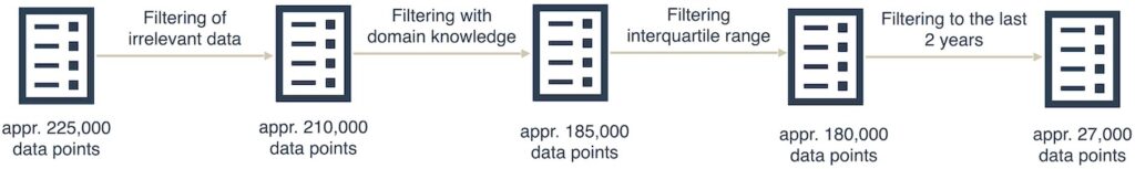
The approach to cleansing the data and training the AI models is based on CRISP-DM. This means that it forms a continuous cycle of business understanding, data understanding, data preprocessing, modeling, evaluation and deployment [5].  This data set was initially exported from the production systems of the cooperating company in CSV format. Later, the data was stored directly in MinIO S3 buckets via a self-developed REST interface, which triggered the corresponding steps for processing the data and training the AI model. The data set contains data from the beginning of 2014 to the end of 2023, with a total of around 225,000 orders distributed across several machines.

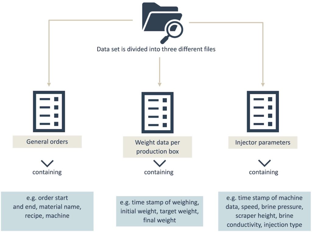
The data set is divided into three files: the first is for the orders, the second for the weight data per production box and the third for the parameters of the brine injector. The files contain the following data: Order start and end, material name, recipe, initial weight (in kg), final weight (in kg), time stamp of weighing and machine data, speed (in T/min), brine pressure (in bars; actual and target), scraper height (in cm; actual and target), brine conductivity (in mS/cm; actual and target) and injection type.

Data preprocessing

In order for the data to be used for the AI models, it must first be merged. This applies to the injector data, which is saved in one file per day and machine. Once the files have been merged, any duplicates are removed. The connection between order and weight data is made via the order number. The connection to the injector parameters is then made via the time stamp of the parameter setting and the start and end of the job. 

The subsequent cleansing of the data set was carried out using domain knowledge from food processing, so that the injector parameters and the weight information corresponded to the value ranges typical for the producer. In addition, entries made irrelevant by production-related breaks such as machine maintenance were removed from the data. Outliers are adjusted using the interquartile range with a threshold of 1.5 [6].

After adjustment, the dataset contains approx. 180,000 entries. The data is then filtered to include only that from the last two years, as prescriptions changed from this period onwards due to legal and customer requirements. After filtering, around 27,000 data points remain that can be used for training and testing the AI models. Figure 2 shows the steps applied. Additional features, such as the weight of the brine and the saturation rate of the meat in each box, were also added. 

So that the AI model can also incorporate categorical values such as the material name, the recipe or the injection type, these are coded and converted into numerical values using Pandas. As there are different spellings for the various materials, a mapping was created to standardize them. The final dataset, which is also used for training the AI models, contains the following features: material name, recipe, initial weight (in kg), speed (in T/min), actual brine pressure (in bars), actual scraper height (in cm) and actual brine conductivity (in mS/cm).

An approach for parameter optimization

This procedure is at odds with the approach used in the literature, where classifications are generally used [6]. Such an approach is not expedient in this case, as the brine weight is given in continuous values and therefore cannot be classified.  Though reinforcement learning, as used in [7], could also be employed, the authors decided against this due to the limited data available.

The chosen approach is to use regression to predict the brine weight per production unit. This is realized via an AI model trained with the material name, recipe, initial weight, scraper height, brine conductivity, injection type and box number to learn which parameters lead to which brine weight. This model is then used to perform parameter optimization. The parameters to be optimized are – depending on production – the speed and the brine pressure. All possible combinations are formed from these, which are narrowed down using domain knowledge from production.

Using brute force, these combinations are entered into the AI model together with the remaining values from the respective order. It is thereby evaluated which combination exhibits the smallest difference to the targeted brine weight. This combination is issued to the employees in cooked ham production as a result.  An alternative option would be to replace the parameter search with a Bayesian optimization in order to gain an advantage in terms of time and performance.

Selection of the evaluation metric

To enable the AI model to learn the relevant correlations, orders that have a higher deviation from the target weight and therefore alter the quality of the product are filtered out. Various filters are used to determine the correct threshold value. So that the individual models can be evaluated, the target/actual deviation of the brine weight is also calculated from the available data, which is denoted by e. The RMSE is used as the key figure, which is calculated as follows: 

(√(mean(e_t² ))

This ensures that the results of the AI model can be interpreted and compared directly in production. The RMSE is also suitable for comparing different approaches [7].

Selection of AI approaches

A simple linear regression model is also used as a benchmark for the performance of the AI models. The other selected models are a random forest, a support vector regression, all from the scikit-learn library [8], two gradient boosting tree models (XGBoost [9] and LightGBM [10]), and an artificial neural network created with Keras [11] and TensorFlow [12]. Before training the individual models, the data is divided into training and test data in a ratio of 9:1. Thus, approximately 22,000 data points are used for training. 

After training, a hyperparameter optimization of the models was carried out. Figure 3 shows the error rates (RMSE) for the test data, without filtering for a target/actual deviation with the optimized models, to ensure comparability of the models and of the different filtering processes. This amounts to 15 kg on the raw data.

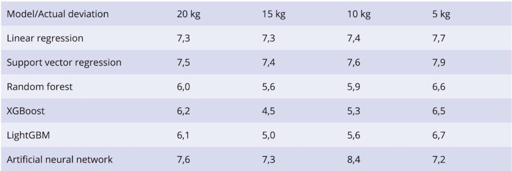
The results of the individual AI models on the test data show that if the filtering is too strong for a small deviation between the target and actual brine weight, the ability of the individual models to abstract new, unseen data decreases significantly. The XGBoost model performs best, with a maximum target/actual deviation of 15 kg. The average error rate here is 4.5 kg, which is less than a third of the average error found in the training data.

From the AI model to production

Once the AI model has been selected, it is implemented in cooked ham production. A WebGUI enables employees to use the AI model. This is carried out using the Streamlit framework, which is well suited to the rapid implementation of prototypes. The individual values of the order can be entered by production employees via the GUI using drop-down fields or sliders.

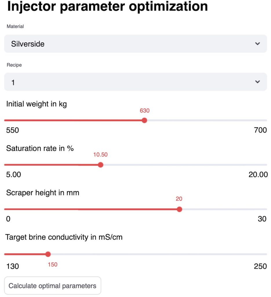
These are then transferred to a server via a REST interface, which calculates the ideal parameters. This functionality can also be transferred and integrated into other programs. So that an evaluation can be carried out in parallel, this is integrated directly into the WebGUI. The data collected in this way is stored in MinIO buckets via the same REST interface and can then be evaluated. Both parts of the solution are provided as containers using Docker [13] and therefore offer good flexibility in terms of the runtime environment and integration in production. At the time of publication, the evaluation has not yet been completed.

Future developments

Once implemented in cooked ham production, the developed AI models help to set the machine parameters on the brine injector in such a way that brine can be dosed in a targeted manner in the corresponding production process. The results of the individual AI models show that the accuracy can be (significantly) increased compared to the current procedure in cooked ham production. Despite the small amount of data of approx. 22,000 data points, it was possible to create a targeted model. 

With the data collection currently underway, the AI model will continuously be exposed to new datasets and can therefore achieve ever better results. The current evaluation is intended to demonstrate the functionality and user-friendliness of the approach. It also evaluates the extent to which the proportion of process-related destructurings in the cooked ham is reduced after using the AI models. The optimization could be further extended to integrate other parameters, such as the brine conductivity.

This would also allow the dosing itself to be optimized with the goal of a more resource-saving production method. In the future, it is conceivable that the AI approaches described here, as well as other AI approaches, could be transferred to additional process steps in cooked ham production. One example of this is the AI-supported visual inspection of delivered meat cuts and the detection of quality-reducing properties such as destructured areas.

This article was created as part of the project “KINLI” (Artificial Intelligence for sustainable food quality in supply chains), which is funded by the Federal Ministry of Food and Agriculture under the grant number 28DK124D20.

You might also be interested in

Optimized Manual Processes in Automotive Production A module-based approach for the efficient creation of work system simulations Barbara Brockmann, Tobias Jurk, Beate Stoffels, Jochen Deuse

In the manufacturing industry, the integration of digital human models into the product development and manufacturing process is becoming increasingly important. Particularly in assembly, which is characterized by a high proportion of manual tasks, motion simulations enable a realistic representation of human work and thus make a significant contribution to the evaluation of motion economy, process validation, and efficiency improvement. However, widespread application in production planning faces various challenges, such as the high initial effort required to create human simulations as well as volatile planning conditions. This article presents a practice-oriented solution from the automotive assembly sector that enables the creation of simulations with reduced effort as well as their early and consistent use in the planning process.

Industry 4.0 Science | Volume 42 | 2026 | Edition 3 | Pages 48-55

AI-Powered Lubrication Strategies for Thread Forming Adaptive spray jet control to increase process reliability and tool life Reinhard Schmied, Marco Susic, Christian Donhauser

Thread forming requires precise lubricant application because high contact pressures and process temperatures strongly influence tool loading, friction, and process stability. Although minimum quantity lubrication (MQL) systems are widely used, current spray-based approaches can still suffer from spray losses, insufficient wetting of the thread grooves, and unstable droplet transport. This article presents a concept for adaptive precision lubrication in thread forming based on computational fluid dynamics (CFD)-supported flow analysis, experimental validation, and artificial intelligence (AI)-assisted optimization. The focus is on droplet size, spray jet geometry, nozzle position, ambient flow conditions, and their influence on wetting intensity. Preliminary simulation-based investigations indicate that data-driven optimization can help identify wetting deficiencies and support the development of future control strategies for resource-efficient lubricant application.

Industry 4.0 Science | Volume 42 | 2027 | Edition 3 | Pages 76-83

SmartBending—Inline Measurement for Process Correction Inline process optimization for error compensation in swivel bending Christian Donhauser , Reinhard Schmied, Marco Susic

Swivel bending is an established forming process that minimizes material loss and enables efficient use of resources. However, the process requires complex optimizations that have traditionally relied heavily on the expertise of machine operators. This results in significant time and material costs, as optimization steps are performed iteratively. Given the shortage of skilled workers, a technological upgrade of the machines in line with Industry 4.0 is necessary. As part of a research project, intelligent sensor technology was used to record critical influencing factors that reveal correlations between product defects and machine deformations. Based on this, a methodology was developed that forms the foundation for inline compensation, enabling the equipment to autonomously adjust process parameters to correct product defects and, in the long term, enable defect-free production from the very first component.

Industry 4.0 Science | Volume 42 | 2026 | Edition 3 | Pages 134-141

Developing Virtual Reality in Learning Contexts Navigating efficiency, content relevance and scalability Stella Kanatouri , Oliver Sosna , Alexander Kulik, Sina C. Truckenbrodt , Friederike Klan , Christian Erfurth

While virtual reality can facilitate hands-on learning, its development faces barriers, including high costs and time demands and scalability challenges. This article presents two case studies that illustrate strategies for overcoming such barriers when training the next generation of skilled workers in environmental technologies. By examining approaches for streamlining development and increasing content relevance and scalability, we highlight lessons learned for future practice. We conclude by envisioning a future in which educational institutions can flexibly and cost-effectively prototype virtual reality in learning contexts, ensuring alignment with curricular goals and learners’ needs.

Industry 4.0 Science | Volume 42 | Edition 3 | Pages 26-34 | DOI 10.30844/I4SE.26.3.3

Industrial Application of Immersive Technologies Exploring XR solutions for training, instruction, design review, and assembly planning Andreas Straube , Faikar Zakky Haidar , Matheus Lenzi dos Santos , Kussai AI Jairoud , Eduardo Koscianski

In recent years, the decreasing cost and improved usability of immersive hardware and software have made extended reality (XR) increasingly attractive for industrial applications. Stand-alone systems with inside-out tracking and camera-based pass-through enable accessible mixed reality (MR) solutions. At the same time, emerging no-code software platforms allow engineers to create XR environments without programming expertise, broadening adoption across production settings. This paper explores key industrial application areas of immersive technologies through selected commercially available XR software solutions for product and process training, spatial instructions and guides, collaborative design review, and assembly and production planning.

Industry 4.0 Science | Volume 42 | 2026 | Edition 3 | Pages 38-47 | DOI 10.30844/I4SE.26.3.4

Learning Factories for the Future of Manufacturing in Brazil Advancing manufacturing through technology and skills development

Manufacturing firms in developing countries face challenges in closing productivity gaps while adopting Industry 4.0 technologies. Learning factories are one helpful approach to countering these challenges. One such example is the learning factory Fábrica do Futuroin São Paulo, Brazil, which has engaged students, supported competence development, and collaborated with industry in applied research, functioning as a hub for advanced manufacturing initiatives.

Bibliography

[1] BMEL: Leitsätze für Fleisch und Fleischerzeugnisse. URL: https://www.bmel.de/SharedDocs/Downloads/DE/_Ernaehrung/Lebensmittel-Kennzeichnung/LeitsaetzeFleisch.pdf?__blob=publicationFile&v=16, accessed 06.08.2024.[2] Brombach C. et al.: Fleischerei heute. 6th edition. Hamburg 2023.
[3] Krämer, J.; Prange, A.: Lebensmittel-Mikrobiologie: 48 Tabellen, 8th edition. In: UTB Lebensmittel- und Ernährungswissenschaften, Biologie, No. 1421. Stuttgart 2023.
[4] Müller Richli, M.; Bee, G.; Stoffers, H.; Scheeder, M.: Strukturfehlern in Schweineschinken auf der Spur. URL: https://www.agroscope.admin.ch/agroscope/de/home/themen/wirtschaft-technik/betriebswirtschaft/publikationen/_jcr_content/par/externalcontent.bitexternalcontent.exturl.html/, accessed 06.08.2024.
[5] Wirth, R.; Hipp, J.: CRISP-DM: Towards a standard process model for data mining. In: Proc. 4th Int. Conf. Pract. Appl. Knowl. Discov. Data Min (January 2000).
[6] Ross, S. M.: Introductory statistics, 3rd edition. Burlington, MA 2010.
[7] Hyndman, R. J.; Koehler, A. B.: Another look at measures of forecast accuracy. In: Int. J. Forecast. 22 (2006) No. 4, pp. 679-688. DOI: 10.1016/j.ijforecast.2006.03.001.
[8] Pedregosa, F. et al.: Scikit-learn: Machine learning in Python. In: J. Mach. Learn. Res. 12 (2011), pp. 2825-2830.
[9] Chen, T.; Guestrin, C.: XGBoost: A Scalable Tree Boosting System. In: Proceedings of the 22nd ACM SIGKDD International Conference on Knowledge Discovery and Data Mining, in KDD ’16, pp. 785-794. New York, NY 2016. DOI: 10.1145/2939672.2939785.
[10] Ke, G. et al.: Lightgbm: A highly efficient gradient boosting decision tree. In: Adv. Neural Inf. Process. Syst. 30 (2017), pp. 3146-3154.
[11] Chollet, F. et al.: Keras. URL: https://github.com/fchollet/keras, accessed 06.08.2024.
[12] Abadi, M. et al.: TensorFlow: Large-Scale Machine Learning on Heterogeneous Systems. 2015. URL: https://www.tensorflow.org/, accessed 06.08.2024.
[13] Merkel, D.: Docker: lightweight linux containers for consistent development and deployment. In: Linux J. (2014) 239, p. 2.
Your downloads
Potentials: Innovation Profitability
Solutions: Production Control Quality Management